Quarterly financial dashboard
Eight KPIs and key accounts in a native Excel dashboard
- Template
- XLSX
- Export as
- XLSX, PDF, ODS, CSV, HTML +19 more
- Carbone
- 5.18+
Generate financial dashboards from your finance system
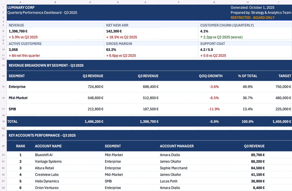
Finance teams and reporting tools send the quarter's figures to the Carbone API as JSON and get back the dashboard as a native Excel file. The generated XLSX keeps the layout of your sheet, its number formats and its conditional formatting, and it stays editable in Excel. Here, a quarterly dashboard presents eight KPIs, the revenue by segment against its target, and the key accounts, with colors that highlight the trends and statuses. The JSON data carries the inputs only: the growth, the share of total, the gap to target, the status and the totals are Excel formulas.
In this example, you will:
- Display KPI cards with amounts and percentages
- Repeat the rows of the segment and account tables
- Compute the growth, the gap to target and the totals with Excel formulas
- Highlight the values with conditional formatting
- Add a dynamic footer
How to build the dashboard in Excel
Follow these steps to generate a financial dashboard:
1. Lay Out the KPI Cards and Tables
In Excel, create a sheet with a header band, eight KPI cards on two lines, a table for the revenue by segment and a table for the key accounts. Each card uses three rows: a label, a value and a trend. In Page Layout > Page Setup, choose the Landscape orientation and fit the sheet on one page wide.
2. Display the Header and the KPIs
Display the data with Carbone tags:
- In the header, mix text and tags in the same cell, for example
{d.report.title} - {d.report.period}orGenerated: {d.report.generatedDate} - Display the amounts with the :formatN formatter, for example
{d.kpis.netNewArr.value:formatN}. In XLSX,:formatNwrites a real number in the cell, and the number format of the cell displays it: set the format#,##0.00 "€"to display1398700as1,398,700.00 € - Display the ratios in the same way, for example
{d.kpis.churnRate.value:formatN}, with the cell format set to Percentage to display0.041as4.1% - Display the trends with
{d.kpis.netNewArr.trend}. The data contains the↑or↓arrow, used to color the text in step 5. The revenue card is a formula,=E18, that reads the total of the segment table
3. List the Segments
Display the segments in a loop:
- In the first row, add
{d.segments[i].name},{d.segments[i].prevRevenue:formatN},{d.segments[i].revenue:formatN}and{d.segments[i].target:formatN} - In the same row, type the formulas:
=E15/C15-1for the growth,=E15/$E$18for the share of total,=E15-I15for the gap to target and=IF(K15>=0,"On Track","Off Target")for the status - In the next row, add
{d.segments[i+1].name}to end the loop - Below, add the TOTAL row with
=SUM(C15:C16)and the same formulas on the total: Carbone updates them to cover every generated row, and the absolute reference$E$18follows the total row
Only style the first row of the loop: Carbone copies its formatting to every generated row.
4. List the Key Accounts
Display the accounts in a loop in the same way, with {d.accounts[i].name}, {d.accounts[i].revenue:formatN}, {d.accounts[i].qoqDelta:formatN}, {d.accounts[i].health}, and so on. In the Rank column, number the accounts with the :cumCount formatter: {d.accounts[i].name:cumCount:formatN}.
5. Add the Conditional Formatting
Carbone keeps the Excel conditional formatting and applies it to the generated values. Go to Conditional Formatting > New Rule... and create the rules:
- Trends: Format only cells that contain > Specific Text
↑in green, and↓in red - Growth and gap to target: Use a formula to determine which cells to format, for example
=G15>0in green and=G15<0in red - Statuses and health: cells containing
On TrackorHealthyin green,Monitorin orange,Off TargetorRiskin red - Banded rows: the formula
=MOD(ROW(),2)=1with a light background
The rows generated by a loop are only formatted inside the range of the rule. Apply the rules to a range that covers the maximum number of rows, for example A23:N1449.
6. Add the Footer
Go to Page Layout > Page Setup > Header/Footer, click Custom Footer..., and type the tags, for example {d.company.name} - Internal Use Only · Source: {d.report.source} · Data as of {d.report.asOfDate}.
Every amount, ratio and rank is a native Excel number, so the generated workbook can be sorted, summed and charted. The currency comes from the number format of the cell, not from the lang and currency options of the API request.
This template requires Carbone v5.18.0 or later. Add the tag
{o.preReleaseFeatureIn=5018000}to the template so the formulas and the conditional formatting follow the generated rows. Here, the tag is stored in the comments of the document properties.
Save the XLSX template, connect it to your JSON data, and let Carbone generate your financial dashboard automatically.
Related Examples
Check out these similar templates to learn more:
Trusted by 800+ paid customers in 40+ countries