Warehouse floor plan heat map
Bay utilization and golden zone slotting moves from your WMS

- Template
- SVG
- Export as
- PDF, PNG, SVG, WebP +24 more
- Carbone
- 5.18+
Generate warehouse heat maps from your WMS
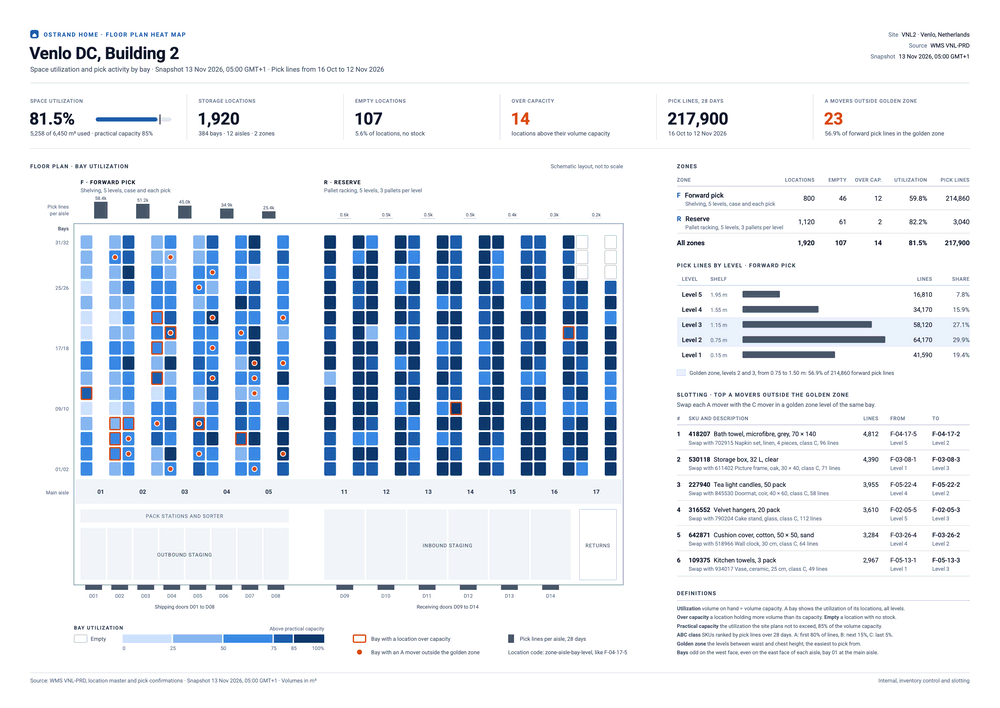
Inventory control teams and slotting analysts review the floor plan of their distribution center every week, and before each peak season: where the racks are full, where locations sit empty or overfilled, and which fast movers are slotted too low or too high. The warehouse management system (WMS) holds the capacity of each location, the stock on hand and the pick confirmations. Your WMS or slotting software sends one record per bay to the Carbone API as JSON, and an SVG template returns an A3 PDF of the floor plan, ready to print for the morning meeting. In this example, the Venlo distribution center of Ostrand Home reviews 1,920 locations and 217,900 pick lines.
In this example, you will:
- Draw the floor plan from the data, one cell for each bay
- Color each bay by its utilization, in five steps
- Flag the bays with a location over capacity or a fast mover outside the golden zone
- Total the utilization and the empty locations of each zone
- Chart the pick lines by level and list the slotting moves
Floor plan layout
The plan follows the slotting rules of Warehouse & Distribution Science (Bartholdi and Hackman, Georgia Tech): rank the SKUs by pick activity in an ABC analysis, and put the most picked SKUs at waist level, in the golden zone. The NIOSH ergonomic guidelines for manual material handling give the same zone for lifting: above the knees, below the shoulders.
| Area | Content | Rule |
|---|---|---|
| Header | Site, source WMS, snapshot time and pick window | The snapshot is taken at 05:00, before the first shift |
| KPIs | Space utilization, locations, empty, over capacity, pick lines, A movers outside the golden zone | Utilization is the volume on hand divided by the volume capacity of all the locations, next to the practical capacity of the site |
| Plan | Forward pick zone F, reserve zone R, main aisle, pack stations, staging lanes and dock doors | Odd bays on the west face of an aisle, even bays on the east face, bay 01 at the main aisle |
| Bay color | Utilization of the 5 locations of the bay: up to 25%, 50%, 75%, the practical capacity, then above it | Empty bays stay white with an outline |
| Alerts | An orange outline for a location over capacity, an orange dot for an A mover outside the golden zone | Each alert has its own shape, so the plan also reads in black and white |
| Pick lines | Per aisle above the plan, and per level in the forward pick zone | The golden zone, levels 2 and 3, is shaded |
| Slotting moves | The 6 most picked A movers outside the golden zone | Each one swaps places with a C mover in a golden zone level of the same bay |
Location codes follow the zone-aisle-bay-level scheme: F-04-17-5 is level 5 of bay 17 in aisle 04 of the forward pick zone.
How to generate a warehouse heat map from WMS data
Follow these steps to build the floor plan template with Carbone:
1. Design the plan on an A3 artboard
- Set the page size on the
svgelement:width="420mm" height="297mm" viewBox="0 0 1190.55 841.89". One unit is one point, and the PDF page takes the size of the SVG. For Tabloid, usewidth="17in" height="11in" viewBox="0 0 1224 792". - Set the fonts once, on the
svgelement:font-family="Roboto, Helvetica Neue, Arial, sans-serif". Roboto is available on Carbone Cloud. On premise, install it on the server. - Draw the fixed parts of the building in your design tool: the walls, the main aisle, the pack stations, the staging lanes and the dock doors. The racks come from the data.
- SVG text does not wrap: the slotting table fits descriptions of about 40 characters.
2. Send one record per bay
The data lists the zones, their aisles and the bays of each aisle, in the order of the bay numbers. Each bay gives the totals of its locations: locations, capacity and used in m³, the number of empty locations, and over and misslotted when they are not zero.
{ "bay": "04", "locations": 5, "capacity": 1.25, "used": 0.92, "empty": 0, "over": 1 }The data also brings the pick lines of each aisle, the pick lines of each level of the forward pick zone, and the list of slotting moves.
3. Compute the utilization of each bay
A comment at the top of the template computes the utilization and the color step of every bay with :set, before the layout:
{d.zones[].aisles[].bays[].used:div(.capacity):set(.fill)}
{d.zones[].aisles[].bays[].fill:ifEQ(0):show(0):ifLTE(0.25):show(1):ifLTE(0.5):show(2):ifLTE(0.75):show(3):ifLTE(d.practicalCapacity):show(4):elseShow(5):set(.bucket)}- The switch case gives each bay the first step whose condition is true: 0 for an empty bay, 5 above the practical capacity, 85% in the data. Change
practicalCapacityin the data: the colors, the legend and the KPI follow. - The bay takes the color of its step:
fill="{d.zones[i].aisles[i].bays[i].bucket:ifEQ(0):show('#FFFFFF'):ifEQ(1):show('#CDE2FB'):ifEQ(2):show('#86B6EF'):ifEQ(3):show('#3987E5'):ifEQ(4):show('#1C5CAB'):elseShow('#0D366B')}". - The darkest step means one thing: above the practical capacity of the site.
4. Draw the racks with nested loops
Three nested loops repeat the group of a zone, the group of an aisle inside it, and the group of a bay inside the aisle:
<g id="zone" transform="translate({d.zones[i].before:mul(50):add(.i * 40 + 96)} 0)">
  <g id="aisle" transform="translate({d.zones[i].aisles[i].aisle:print(..i):mul(50)} 0)">
<g id="bay" transform="translate({d.zones[i].aisles[i].bays[i].bay:print(...i):mod(2):mul(34)} {d.zones[i].aisles[i].bays[i].bay:print(...i):div(2):floor:mul(-18)})">...iis the number of the bay in its aisle. :mod puts the odd bays on the west face and the even bays 34 points to the right, on the east face. :floor gives the row, and each row moves 18 points up from the main aisle. See the loop index...iis the number of the aisle in its zone: each aisle is 50 points wide, a rack face, the aisle, the other rack face and the flue between two back-to-back racks.beforecounts the aisles of the previous zones, so a zone can hold any number of aisles. The comment computes it:{d.zones[].aisles[].aisle:aggCount(.i):set(..aisleCount)}, then{d.zones[].aisleCount:cumSum:sub(.aisleCount):set(.before)}.- A group with
{d.zones[i].aisles[i].bays[i+1].bay}closes the loop of the bays, and the same groups withaisles[i+1]andzones[i+1]close the two other loops.
5. Flag the exceptions
The outline and the dot of each bay are in the template, and their display attribute shows them only when the bay has an exception:
display="{d.zones[i].aisles[i].bays[i].over:ifGT(0):show('inline'):elseShow('none')}"A bay without over in the data hides its outline. The dot uses misslotted the same way.
6. Total each zone and the site
Aggregators grouped by zone store the totals in each zone, and the comment adds them up for the site:
{d.zones[].aisles[].bays[].used:aggSum(.i):set(...used)}
{d.zones[].aisles[].bays[].capacity:aggSum(.i):set(...capacity)}
{d.zones[].used:aggSum:set(c.used)}
{d.zones[].capacity:aggSum:set(c.capacity)}(.i)groups the bays by zone, and...usedwrites the total in the zone, two levels above the bay. The same tags total the locations, the empty and the over-capacity locations, and the pick lines.- The KPI divides the two totals:
{c.used:div(c.capacity):mul(100):formatN(1)}%prints 81.5%. The zone table loops on the zones and prints{d.zones[i].used:div(.capacity):mul(100):formatN(1)}%. - The total row of the table moves under the last zone:
transform="translate(0 {d.zones[].code:aggCount:mul(28)})".
7. Chart the pick lines by level and list the moves
- Each bar of the level chart is 170 points long for the busiest level:
width="{d.levels[i].lines:div(c.levelPeak):mul(170)}", wherec.levelPeakstores{d.levels[].lines:aggMax}. - The levels of the golden zone have
"golden": 1in the data. A filter totals their pick lines:{d.levels[golden=1].lines:aggSum:set(c.goldenLines)}, and the KPI prints their share, 56.9%. - The slotting table shows the first 6 moves of the list:
{d.moves[i, i < 6].sku}. Your slotting software sends them sorted by pick lines. - The last character of a location code is its level:
Level {d.moves[i, i < 6].from:substr(-1)}prints Level 5 for F-04-17-5.
8. Generate the PDF
Send the data with these options:
{
  "data": { ... },
  "convertTo": "pdf",
  "converter": "C",
  "lang": "en-gb",
  "timezone": "Europe/Amsterdam"
}
"converter": "C"draws the SVG with Chrome. The PDF has one A3 page, with vector shapes and selectable text.timezoneprints the snapshot time of the site:{d.asOf:formatD('D MMM YYYY, HH:mm z')}prints 13 Nov 2026, 05:00 GMT+1.- To show the plan on a screen in the warehouse office, ask for a PNG:
"convertTo": { "formatName": "png", "formatOptions": { "Scale": 2 } }. See Convert SVG to PNG or PDF. - Call the API every morning after the WMS snapshot, with one request for each building or site.
SVG templates require Carbone v5. The conversion of an SVG to PDF with Chrome requires Carbone v5.17.0 or later.
Related Examples
Trusted by 800+ paid customers in 40+ countries