Monthly treasury FX report
Daily ECB rates, monthly averages and statistics against the budget rate
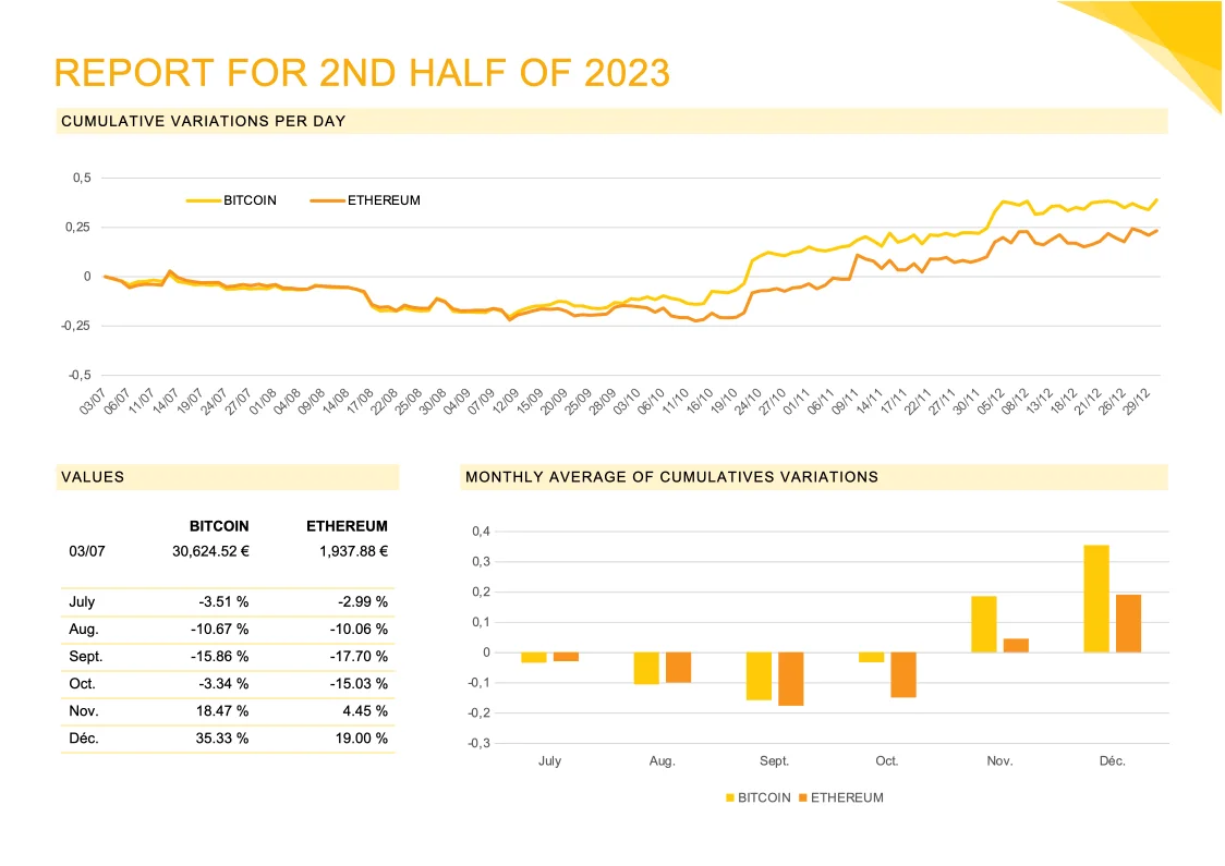
- Template
- DOCX
- Export as
- PDF, DOCX, ODT, HTML, PNG +25 more
- Carbone
- 5.0+
Generate treasury FX reports from your market data
Group treasury teams send the month's exchange rates to the CFO and the risk committee: the closing rate for the balance sheet, the monthly average for the income statement (an average rate that IAS 21 accepts when rates do not fluctuate significantly), and the gap with the budget rate. Your treasury management system or market data feed sends the daily rates to the Carbone API as JSON, and a DOCX template draws native Word charts and fills the statistics table.
In this example, Arvenne Industries, a fictional European group with US dollar sales, reports EUR/USD for October 2026. The data holds the real euro reference rates of the European Central Bank from January to October 2026; the budget rate, the hedging figures and the commentary are fictional.
In this example, you will:
- Draw a line chart from the daily rates, on a date axis
- Draw a column chart from the monthly averages, with the budget rate as a line
- Print the last item of an array
- Compute changes and gaps to the budget in the template
How to draw FX charts from JSON in a Word report
Follow these steps to add native charts and statistics to your report:
1. Prepare the JSON Data
Send the daily rates, the monthly averages, the budget rate and the statistics of the month and of the year to date. Your system computes the statistics from the same daily series: the opening rate (the last rate of the previous period), the high and low with their dates, the average, and the volatility, the annualised standard deviation of daily log returns.
{
  "budgetRate": 1.15,
  "rates": [
    { "date": "2026-01-02", "rate": 1.1721 },
    { "date": "2026-01-05", "rate": 1.1664 }
  ],
  "months": [
    { "month": "2026-01-01", "average": 1.1738, "observations": 21 }
  ],
  "stats": {
    "month": { "openingDate": "2026-09-30", "opening": 1.1355, "high": 1.1298, "highDate": "2026-10-01",
               "low": 1.113, "lowDate": "2026-10-29", "average": 1.1202, "volatility": 0.0528, "observations": 22 },
    "ytd":   { "openingDate": "2025-12-31", "opening": 1.175, "average": 1.1568, "volatility": 0.0558 }
  }
}
2. Add a Line Chart on a Date Axis
Insert a Line chart at the top of the report. Right-click it, select Edit Data in Excel, and define the loop on the rates array:
|                                                               | EUR/USD             | Budget rate                             |
|---------------------------------------------------------------|---------------------|-----------------------------------------|
| {d.rates[i].date:formatD(X):div(86400):add(25569):round(0)}   | {d.rates[i].rate}   | {d.rates[i].rate:print(..budgetRate)}   |
| {d.rates[i+1].date:formatD(X):div(86400):add(25569):round(0)} | {d.rates[i+1].rate} | {d.rates[i+1].rate:print(..budgetRate)} |- Word and Excel store a date as a number of days since 30 December 1899. :formatD(X) returns the Unix timestamp in seconds, :div turns it into days, :add moves the origin to 1899 and :round keeps whole days.
- Right-click the horizontal axis, select Format Axis, choose Date axis, set the major unit to 1 month and the number format to
mmm: the axis shows one label per month, whatever the number of rates in the month. - :print(..budgetRate) prints the
budgetRateattribute found one level above theratesarray on every row, which draws the budget rate as a flat line. Format it as a dashed line.
3. Add a Column Chart of the Monthly Averages
Insert a Clustered Column chart and define the loop on the months array:
|                                    | Monthly average         | Budget rate                                 |
|------------------------------------|-------------------------|---------------------------------------------|
| {d.months[i].month:formatD(MMM)}   | {d.months[i].average}   | {d.months[i].average:print(..budgetRate)}   |
| {d.months[i+1].month:formatD(MMM)} | {d.months[i+1].average} | {d.months[i+1].average:print(..budgetRate)} |
Then:
- Right-click the Budget rate series, select Change Series Chart Type and choose Line.
- Add data labels to the columns with the number format
0.0000. - Set the minimum of the vertical axis to
1.10, so the gaps between months stay readable.
4. Print the Closing Rate
The closing rate is the last item of the rates array: a negative index reads it without a loop.
{d.rates[i=-1].rate:formatN(4)}prints 1.1172: :formatN(4) keeps the 4 decimals used to quote EUR/USD.{d.rates[i=-1].date:formatD('D MMMM YYYY')}prints 30 October 2026.
5. Compute Changes in the Template
Compute the change of the month from the closing rate and the opening rate: {d.rates[i=-1].rate:div(d.stats.month.opening):sub(1):mul(100):formatN(2)}% prints -1.61%. Insert {d.rates[i=-1].rate:div(d.stats.month.opening):sub(1):mul(100):ifGT(0):show('+'):elseShow('')} just before it to add a plus sign to a rise.
The same pattern compares the averages with the budget rate, for example {d.stats.month.average:div(d.budgetRate):sub(1):mul(100):formatN(1)}% for -2.6%. In the statistics table:
{d.stats.month.high:formatN(4)}with its date below,{d.stats.month.highDate:formatD('D MMM')};{d.stats.month.volatility:mul(100):formatN(1)}%for the volatility;- the same tags with
ytdinstead ofmonthin the Year to date column.
6. Add the Commentary and the Disclaimer
Write {d.commentary[i].text} in a paragraph and {d.commentary[i+1].text} in the next one: Carbone repeats the paragraph for each comment. End with {d.disclaimer}, the note that states the source of the rates and the internal use of the report.
Tip: set lang to en-gb in your API request to print dates such as 30 October 2026 and numbers with a decimal point.
Save the DOCX template, connect it to your rates, and let Carbone produce the report every month.
Related Examples
Trusted by 800+ paid customers in 40+ countries